Introduction

One of the more unique student sections in college basketball belongs to the Arizon State Sun Devils and their famous “Curtain of Distraction”. The Curtain of Distraction opens to reveal students in ridiculous attire trying to do all they can to break the focus of opposing free throw shooters. Perhaps the most famous attempted distraction occured when Olympic swimmer Michael appeard from behind the curatin wearing only a speedo. Several outlets claim anecdotally that Curtain of Distraction works but don’t offer statistical evidence. Justin Wolfers of The Upshot attempted to quantify the effect of the Curtain of Distraction and found it to increase ASU’s home court advantage by 1-2 points.

Is the advantage still present (Wolfer’s article was written 4 years ago)? Let’s take a look, using my ncaahoopR R package.

Exploratory Analysis

We’ll first just look at which teams ASU has played at home and how they have faired from the charity stripe in Tempe. We begin by first scraping data for all of Arizona State’s home games for the 2018-19 season.

library(ncaahoopR)

### Get Arizona State's Home Games for 2018-19 Season
asu_home_games <- 
  get_schedule("Arizona State") %>%
  filter(date <= Sys.Date(), location == "H")

### Get Arizona State's Roster
asu_roster <- get_roster("Arizona State")

### Get play by play data for all of Arizona State's home games this year
pbp_data <- get_pbp_game(asu_home_games$game_id)

Next, we can tag free throws as made/missed and by which team attempted the free throw.

### Extract Free Throws
free_throws <- filter(pbp_data, grepl("Free Throw", description))

### Tag Free Throw Team
free_throws$ft_team <- NA
for(i in 1:nrow(free_throws)) {
  free_throws$ft_team[i] <- 
    case_when(any(sapply(asu_roster$name, grepl, free_throws$description[i])) ~ 
                free_throws$home[i],
              T ~ free_throws$away[i])
}
free_throws$made <- grepl("made", free_throws$description)

Next, we’ll aggregate the results. Since play-by-play data isn’t availble for Arizona State’s home contest against Oregon State, I’ve manually added the free throw stats from that game.

sum_stats <- 
  group_by(free_throws, ft_team) %>%
  summarise("n_made" = sum(made),
            "n_attempts" = n(),
            "ft_pct" = mean(made)) %>%
  ungroup() %>%
  filter(ft_team != "Arizona State") %>%
  bind_rows(tibble("ft_team" = "Oregon State", "n_made" = 13, 
                   "n_attempts" = 20, "ft_pct" = 0.65)) %>%
  arrange(desc(ft_pct))
knitr::kable(sum_stats)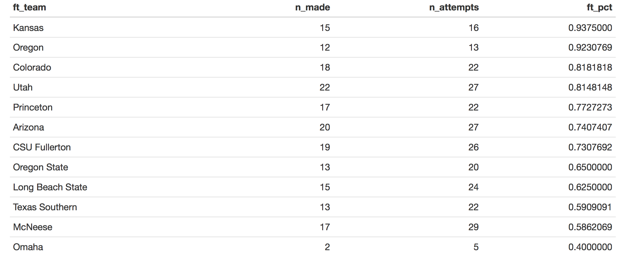

A More In-Depth Look

Of course, these numbers don’t mean much in context. Perhaps Kansas is a really good free throw shooting team or McNeese is a really bad free throw shooting team to begin with. What we are really interested in is how team’s free-throw shooting differs from their season-average when they play against Arizona State. Specifically, we’ll look at home a team’s season-averge FT% in other true road compares to road games at ASU.

### Loop over ASU Home Opponent
for(i in 1:nrow(asu_home_games)) {
  ### Get ESPN Name of ASU Home Opponent
  opp <- dict$ESPN[dict$ESPN_PBP == asu_home_games$opponent[i]]
  if(length(opp) == 0) {
    opp <- asu_home_games$opponent[i]
  }
  if(opp == "McNeese") {
    opp <- "Mcneese"
  }
  if(opp == "Long Beach State") {
    opp <- "Long Beach St"
  }
  
  ### Get Opponent's PBP Data 
  opp_away_pbp <- 
    get_schedule(opp) %>%
    filter(date <= Sys.Date(), location == "A") %>%
    pull(game_id) %>%
    get_pbp_game()
  opp_roster <- get_roster(opp)
  
  ### Tag Free Throws
  opp_free_throws <- filter(opp_away_pbp, grepl("Free Throw", description))
  opp_free_throws$ft_team <- NA
  for(i in 1:nrow(opp_free_throws)) {
    opp_free_throws$ft_team[i] <- 
      case_when(any(sapply(opp_roster$name, grepl, opp_free_throws$description[i])) ~ 
                  opp_free_throws$away[i],
                T ~ opp_free_throws$home[i])
  }
  if(opp == "Mcneese") {
    opp <- "McNeese"
  }
  if(opp == "Long Beach St") {
    opp <- "Long Beach State"
  }
  opp_free_throws <- filter(opp_free_throws, ft_team == opp)
  opp_free_throws$made <- grepl("made", opp_free_throws$description)
  
  ### Aggregate Game by Game Opponent FT Stats
  opp_season_stats <- 
    group_by(opp_free_throws, home) %>%
    summarise("n_made" = sum(made),
              "n_attempts" = n(),
              "ft_pct" = mean(made)) %>%
    ungroup() %>%
    mutate("team" = opp)
  
  ### Save Results
  if(!exists("ft_stats")) {
    ft_stats <- opp_season_stats
  }else{
    ft_stats <- bind_rows(ft_stats, opp_season_stats)
  }
}

ft_stats <- bind_rows(ft_stats, tibble("home" = "Arizona State", "n_made" = 13, 
                                       "n_attempts" = 20, "ft_pct" = 0.65, "team" = "Oregon State"))

Let’s plot free throw shooting by game and visually see what’s going on.

ggplot(ft_stats, aes(x = ft_pct, y = team)) +
  geom_point(aes(color = (home != "Arizona State"))) +
  theme_bw() +
  theme(legend.position  = "bottom",
        plot.title = element_text(size = 16, hjust = 0.5),
        plot.subtitle = element_text(size = 12, hjust = 0.5),
        axis.title = element_text(size = 14)) +
  labs(x = "Free Throw Percentage",
       y = "Team", 
       col = "Home Team",
       title = "Arizona State Opponent's Free Throw Shooting",
       subtitle = "True Road Games Only") +
  scale_color_manual(values = c(ncaa_colors$secondary_color[ncaa_colors$espn_name == "Arizona State"], 
                                ncaa_colors$primary_color[ncaa_colors$espn_name == "Arizona State"]),
                     labels = c("Arizona State", "Other"))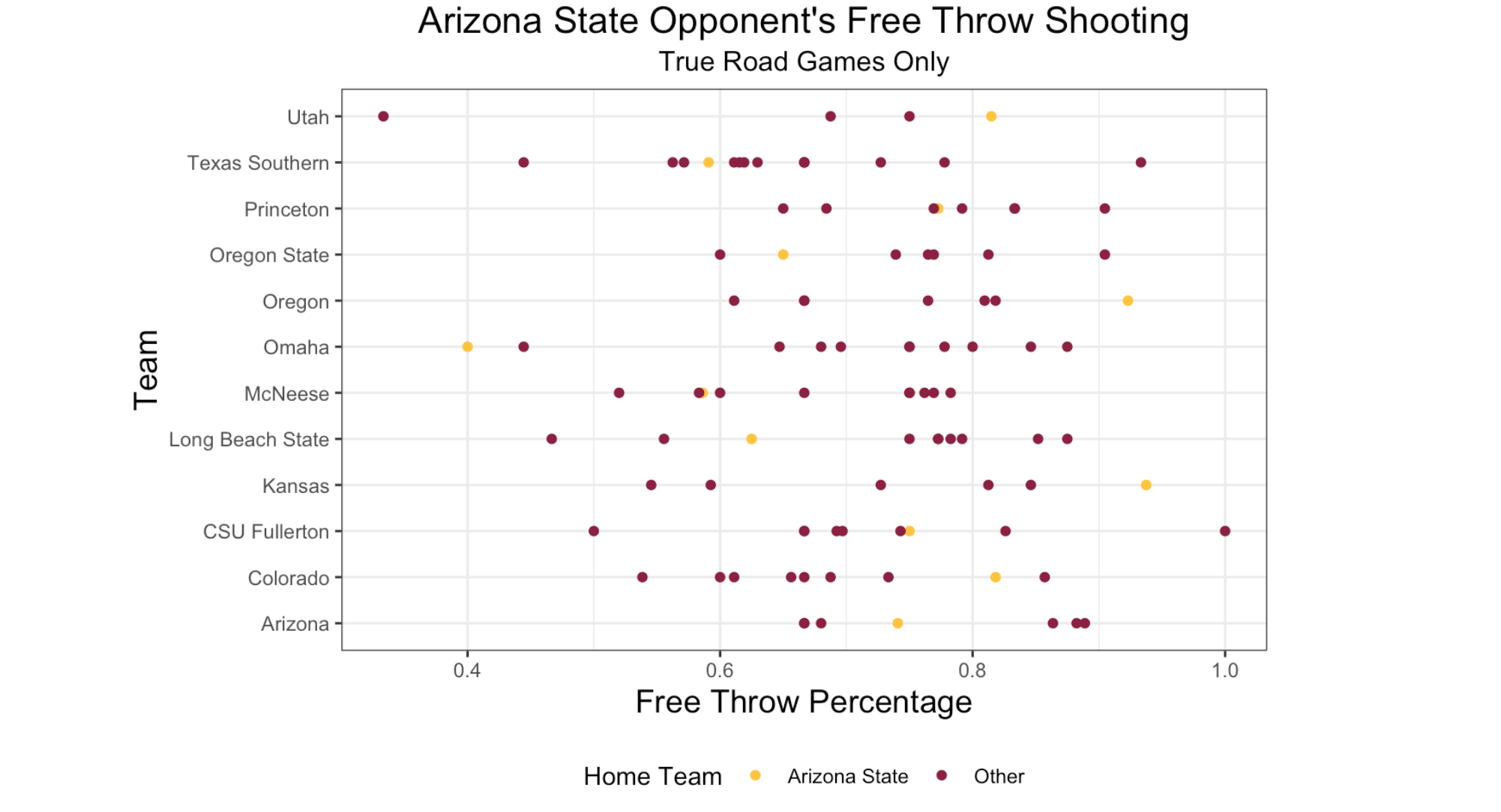

A few play-by-play logs are not available on ESPN, but we have more than enough games to suggest that the effect of the Curtain of Distraction is reduced this year. Three teams had their best road FT shooting performance against the Sun Devils, while the majority of the others seem to fall within the reasonable range one would expect given their other performances. In fact, we can actually quantify how likely each shooting performance at ASU was. Assume that the number of free on opponent took against Arizona State follows a binomial\((n,p)\) distribution where \(n\) denotes the number of free throw attempts against ASU and \(p\) denotes the percentage of free throws that opponent missed in it’s other true road games. We then get the likelihood of each shooting performance against ASU as follows:

season_ft_stats <- 
  filter(ft_stats, home != "Arizona State") %>%
  group_by(team) %>%
  summarise("n_made" = sum(n_made),
            "n_attempts" = sum(n_attempts),
            "ft_pct" = n_made/n_attempts) %>%
  ungroup()

p_performance <- rep(NA, nrow(season_ft_stats))
p <- rep(NA, nrow(season_ft_stats))
n_miss <- rep(NA, nrow(season_ft_stats))
n_attempts <- rep(NA, nrow(season_ft_stats))
for(i in 1:nrow(season_ft_stats)) {
  opp <- season_ft_stats$team[i]
  game <- filter(ft_stats, home == "Arizona State", team == opp)  
  n_miss[i] <- game$n_attempts - game$n_made
  n_attempts[i] <- game$n_attempts
  p[i] <- 1 - season_ft_stats$ft_pct[season_ft_stats$team == opp]
  p_performance[i] <- 1 - pbinom(n_miss[i] - 1, n_attempts[i], p[i])
}

tibble("team" = season_ft_stats$team,
       "p_value" = p_performance) %>%
  arrange(desc(p_value)) %>%
  knitr::kable()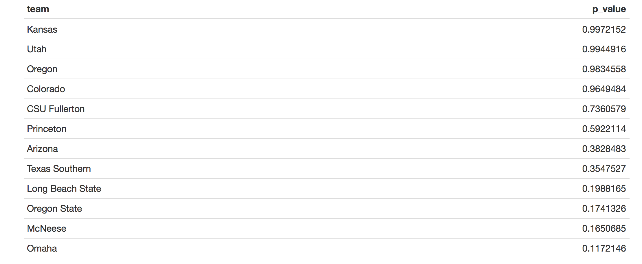

We see that none of the 12 opponent shooting performances differ from those teams’ normal road free throw shooting behavior in a statistically significant manner. That is to say, there is no evidence to suggest the Curtain of Distraction has had any major impact on opponent free throw shooting this season. We can see this visually in the below graphic.

set.seed(123)
for(i in 1:nrow(season_ft_stats)) {
  df <- tibble("miss" = rbinom(100000, n_attempts[i], p[i]),
               "team" = season_ft_stats$team[i],
               "n_miss" = n_miss[i])
  if(i == 1) {
    sim_results <- df
  }else{
    sim_results <- bind_rows(sim_results, df)
  }
}

ggplot(sim_results, aes(x = miss)) +
  facet_wrap(~team) +
  geom_histogram(bins = 23, aes(fill = team)) +
  geom_vline(data = .%>% group_by(team) %>% summarise("miss" = max(n_miss)),
               aes(xintercept = miss), lty = 2) +
  theme_minimal() +
  theme(legend.position  = "none",
        plot.title = element_text(size = 16, hjust = 0.5),
        plot.subtitle = element_text(size = 12, hjust = 0.5),
        axis.title = element_text(size = 14),
        axis.text.y = element_blank()) +
  labs(x = "Free Throws Missed",
       y = "Frequency",
       title = "Expected Distributions of Missed Free Throws Against ASU",
       subtitle = "Under Null Hypothesis of No Curtain Effect") +
  scale_fill_manual(values = c("#CC0033", "#CFB87C", "#00274C", "#0051BA",
                               "#FFC72A", "#FDD023", "#000000", "#154733", "#DC4405",
                               "#FF671F", "maroon", "#CC0000"))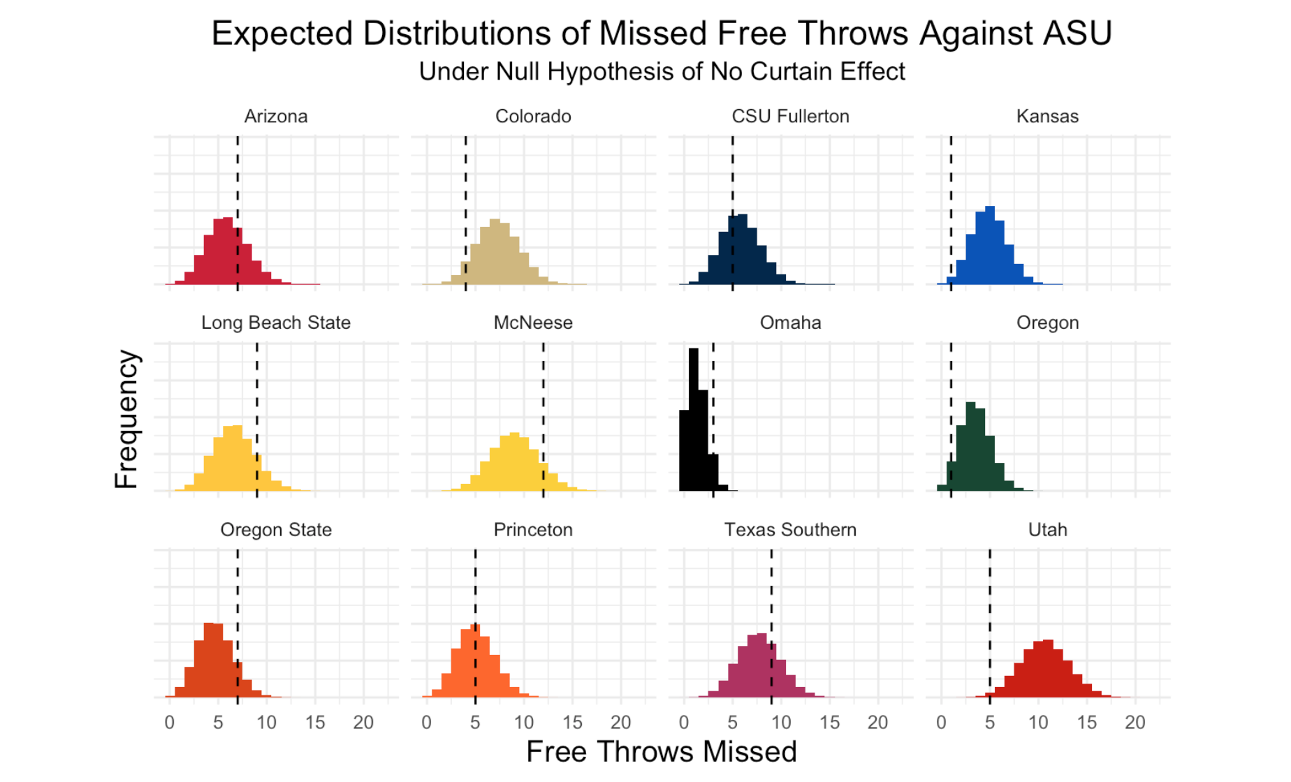

Conclusion

There is strong evidence to suggest that the Curtain of Distraction isn’t doing much to distract opposing free throw shooters this year. This differs from the conclusion of the Upshot piece from several years ago, but doesn’t necessarily contradict it. At the time of the Upshot article, the Curtain of Distraction had only been in existence for two years. Now, four years later, Pac 12 opponents have faced the student section several times, and teams perhaps now know what to prepare for. In any case, future research will examine when such a decline in the significance of distracting took place, and whether the trend has been on a steady decline over the last four years or whether this year is somewhat of a statistical fluke.