Introduction
For the past two years, I’ve been maintaining a men’s college basketball prediction model that I first built for the Yale Undergraduate Sports Analytics Group (YUSAG) during my sophomore year of college. The model has done objectively quite well over the past two seasons. It correctly predicted last year’s National Champion, Villanova, and accurately predicted North Carolina and Gonzaga as the most likely finalists in the 2017 title game. Brackets filled out using model derived predictions have finished above the 90th percentile on ESPN each of the past two seasons. Using my model, I even won the 2018 American Statsitical Association Statsketball Tournament. Having two seasons of experience with this project under my belt, there are a number of additional features I’ve been interested in adding/changing for the 2018-19 season.
Background
Before we get into what’s different this year, we need to look at the way the YUSAG model has worked in the past. The core of the model is linear regression, specified by \[ Y = \beta_{team}X_{team} - \beta_{opp}X_{opp} + \beta_{loc}X_{loc} + \epsilon \]
where \(X_{team, i}, X_{opp, i}\), and \(X_{loc, i}\) are indicator vectors for the \(i^{th}\) game’s team, opponent, and location (Home, Away, Neutral) from the perspective of team, and \(Y_i\) is game’s the score-differential. The key assumptions for this model are that game outcomes are independent of one another, and that our error \(\epsilon \sim N(0, \sigma^2)\).
\(\beta_{team}\), nicknamed “YUSAG Coefficients”, were scaled to represent the points better or worse a team was the average college team basketball team on a neutral court. Lastly, \(\beta_{loc}\) is a parameter indicating home-court advantage, estimated to be about 3.2 points.
Note that the coefficients \(\beta_{opp}\) have the same values and interpretation as \(\beta_{team}\). I’ll note that when this model is actually fit, \(\beta_{opp} = -\beta_{team}\) but in the interest of easy interpretation in these methodology notes, I have flipped the signs of the \(\beta_{opp}\) coefficients and added a minus sign to the model formulation above.
Let’s walk through an example to see how this all works. Say Yale is hosting Harvard, and we’d like to predict score differential. \(\widehat\beta_{team = Yale} = -2.1\) and \(\widehat\beta_{opp = Harvard} = 1.9\). This means that on a neutral court, Yale is 2.1 points worse than the average college basketball team, and Harvard is 1.9 point better. Our predicted outcome for this game would be as follows: \[ \widehat Y_i = \widehat \beta_{team = Yale} - \widehat \beta_{opp = Harvard} + \widehat \beta_{loc = Home} = -2.1 - 1.9 + 3.2 = -0.8 \] Hence, we’d expect Harvard to win this game by roughly 0.8 points. Of course, we could’ve predicted the game from the perspective of Harvard as well, and we’d get exactly the same answer. Since \(\beta_{opp = Yale} = \beta_{team = Yale}\) and \(\beta_{team = Harvard} = \beta_{opp = Harvard}\), we have \[ \widehat Y_i = \widehat \beta_{team = Harvard} - \widehat \beta_{opp = Yale} + \widehat \beta_{loc = Away} = 1.9 - (-2.1) - 3.2 = 0.8 \]
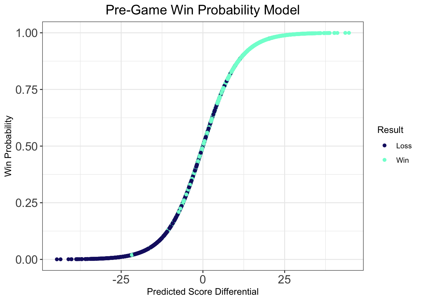
We recover the Harvard by 0.8 predicted scoreline, and hence, it doesn’t matter which school we use as “team” or “opponent” because the results are identical. Once we have a predicted score differential, we can convert this to a win probability using logistic regression. I won’t get into the specifics how logistic regressions works in this post, but for the purposes of this example, just think about it as a translation between predicted point spread and predicted win probability.
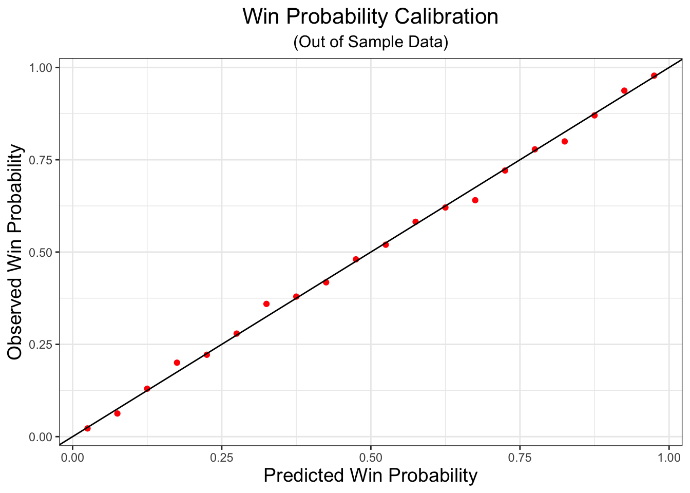
One thing that we check to see is that the win probability model is well calibrated. That is, if we predict a team has a 75% chance of winning, then we should see them win about 75% of the time on out of sample data. To see that the model is well tuned, I’ve fit the logistic regression on data from the 2017-18 season, and then made predictions of win probability from prior predicted score differentials for the 2016-17 season. We don’t see any drastic deviations from the line denoting perfect correspondence between predcited and observed win probability. This is good–it means teams are winning about as often as we predict they are winning!
Offense and Defense Specific Models
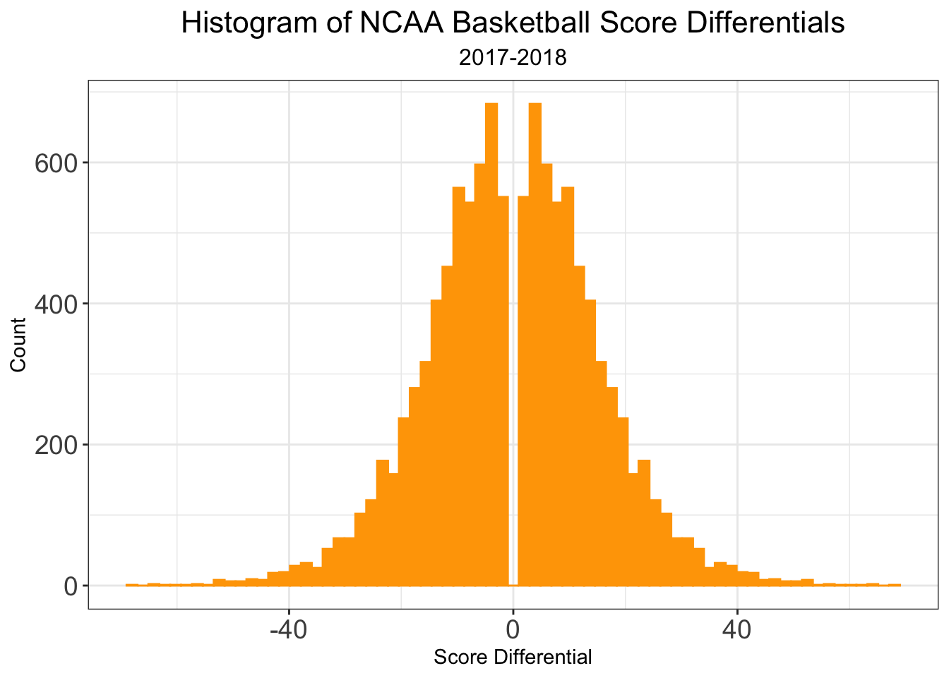
Now that we have the basics of model, we can dive into what’s new for this season. In the past, I’ve only been interesting in predicting game score differential, \(Y_i\). In fact, we can rewrite score differentials as \(Y_i = T_i - O_i\), where \(T_i\) denotes team_score and \(O_i\) denotes opp_score for game \(i\), respectively. Not only is the distribution of score_differential normally distributed, but so too is the distribution of team_score. I’ll note that the gap around 0 in the distribution of score_differential is due to the fact that games can’t end in ties. I’ll also comment that the distribution of opp_score is identical to that of team_score as each game is entered twice in the database, so there is a direct one-to-one correspondence between each value of team_score and opp_score.
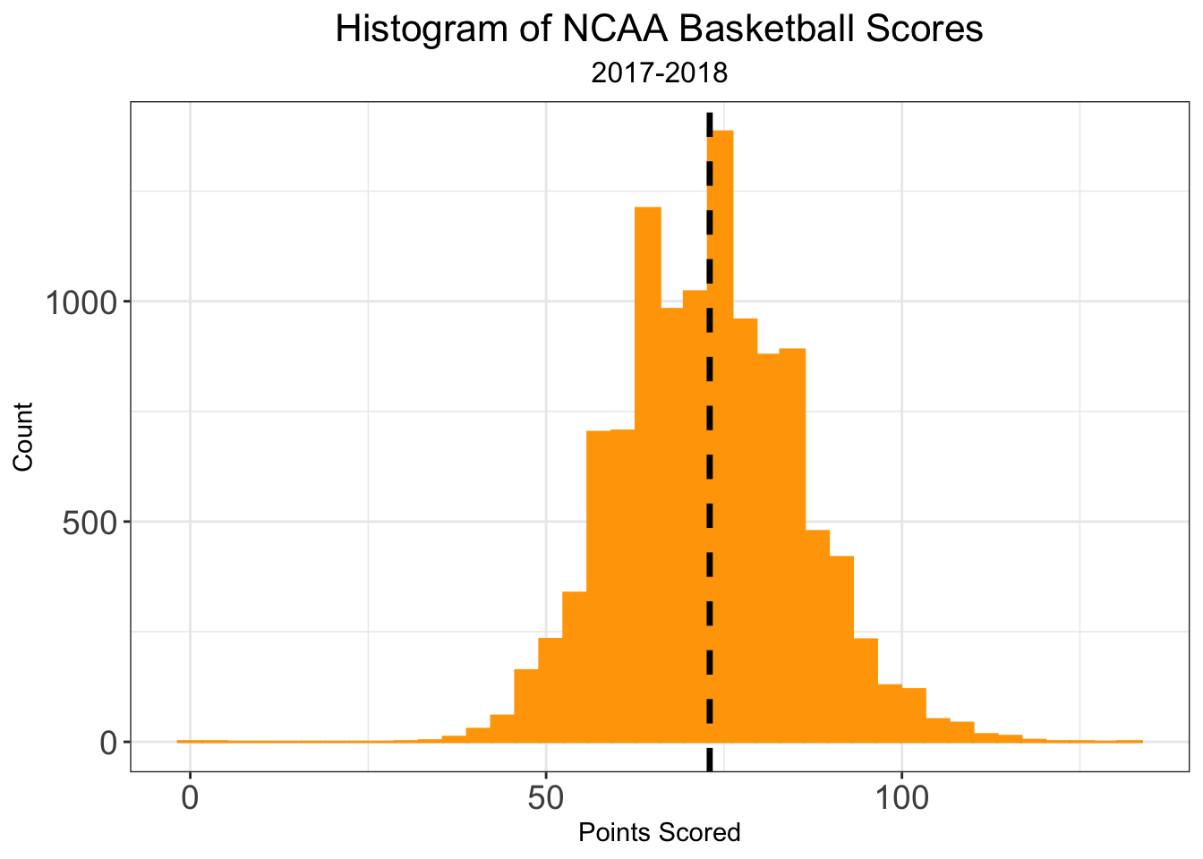
Recall, the sum of two normal random variables is also normally distributed, even if they are not indepent of one another. Thus, using the same linear model framework, we can predict for each game \(T_i\) and \(O_i\). That is, in addition to a predicted score differential, we can actually predict the number of points each team will score. As a consqeuence, we can obtaining estimates of team offensive and defensive coefficeints, \(\alpha_{team}\) and \(\delta_{team}\), respectively. To be clear, this is not necessarily a different model, but a reparameterization that allows us to learn more informations about the contributions of team strength.
\[ Y = \beta_{team}X_{team} - \beta_{opp}X_{opp} + \beta_{loc}X_{loc}\\ (T - O) = \beta_{team}X_{team} - \beta_{opp}X_{opp} + \beta_{loc}X_{loc} \\ T - O = (\alpha_{team} - \delta_{team})X_{team} - (\alpha_{opp} - \delta_{opp})X_{opp} + \beta_{loc}X_{loc} \\ T - O = (\alpha_{team} - \delta_{team})X_{team} - (\alpha_{opp} - \delta_{opp})X_{opp} + \beta_{loc}X_{loc} + (\beta_0 - \beta_0) \\ \] Specifically, we can split the above equation into the following two equations \[ T = \beta_0 + \alpha_{team}X_{team} - \delta_{opp}X_{opp} + \beta_{loc, off}X_{loc}\\ O = \beta_0 -\delta_{team}X_{team} + \alpha_{opp}X_{opp} + \beta_{loc, def}X_{loc} \] where \(\beta_{loc, off}\) and \(\beta_{loc, def}\) denote the contributions to home court advantage to offense and defense, respectively, and \(\beta_0\) is the average number of points scored (for one team) per game across all of college basketball, roughly 73 points. So what is this actually saying? For a given game we predict \(T\), the number of points a team will score by
- Begin with the baseline average number of points scored, \(\beta_0\)
- Add a team specific offensive term, \(\alpha_{team}\). We can interpret \(\alpha_{team}\) as the number of points more than the baseline (\(\beta_0\)) our desired team would score against the average college basketball team on a neutral floor.
- Subtract an opponent specific defensive term, \(\delta_{opp}\). We can interpret \(\delta_{opp}\) as the number of points fewer than the baseline (\(\beta_0\)) our desired team’s opponent would allow against the average college basketball team on a neutral floor.
- Add an term to adjust for home court advantage.
By symmetry, our prediction of the number of points our desired team allows, \(O\), is calculated in almost exactly the same way. Perhaps the math unnecessarily overcomplicates something fairly straightforward, but I think that the derivation of these formulae show how these offensive and defensive coefficients should be interpreted. It’s easy to want to interpret these as meaures of offensive and defensive strength, but it’s extremely important we don’t fall for this temptation. Rather, we should view \(\beta_{team}\) as estimates of overall team strength, and \(\alpha_{team}\) and \(\delta_{team}\) as indicators of how teams derive their strength. For example, consider the top six teams from the end of the 2017-18 season by offensive and defensive coefficients.
Top \(\alpha_{team}\)
##             team off_coeff def_coeff yusag_coeff overall_rank
## 1      Villanova  17.98007  7.946133    25.92621            1
## 2       Oklahoma  15.84885 -4.138373    11.71048           43
## 3           Duke  15.42955  7.892312    23.32186            2
## 4 North Carolina  14.85430  3.956107    18.81041            8
## 5         Xavier  14.26454  2.986246    17.25079           13
## 6         Kansas  12.73801  6.421469    19.15948            7
Top \(\delta_{team}\)
##         team off_coeff def_coeff yusag_coeff overall_rank
## 1   Virginia -2.383885  23.25942    20.87554            5
## 2 Cincinnati  2.420159  16.90140    19.32156            6
## 3   Syracuse -2.952363  14.43724    11.48487           45
## 4   Michigan  4.521445  14.09245    18.61390            9
## 5 Texas Tech  4.553551  13.00919    17.56274           11
## 6  Tennessee  5.024089  12.07138    17.09547           14
We see the pitfall of interpreting \(\alpha_{team}\) and \(\delta_{team}\) as direct measures of offensive and defensive strength most noticably in the case of Virginia. We might be tempted to say that Virgina had a below average offense in 2017-18. This is not exactly the case. On a points per game basis, UVA scored fewer points than the average college basketball team, but this is because their elite defense would often slow down the game, leaving fewer possessions for their offense to score. Adjusted for tempo, UVA had a top-25 offense last season. Their overall team strength is nicely captured by their YUSAG Coefficient, \(\beta_{team}\). \(\alpha_{team}\) and \(\delta_{team}\) illustrate that Virginia derives it’s strength from suffocating defense, but shouldn’t be used to rank teams offensively and defensively, at least not in a vaccuum. If one feels so inclined to utilize \(\alpha_{team}\) and \(\delta_{team}\) to comment about an individual team’s offense and defense, they might look at the difference between the two coefficients in an attempt to quantify team balance and see which facet of the game, if any dominates, team play. For example, compare Virginia’s defense first style of play with the more balanced approaches of Villanova, Duke, and Kansas. Not adjusting for tempo is not problematic provided that we are clear on the subtleties of interpreting the model coefficients. This is a big enough point that I’ll repeat it again:
- Only \(\beta_{team}\) should be used when ranking teams based on team strength. These coefficients CAN be used to make statements such as, “Duke is the best team”, and “the average Ivy League team is worse than the average team from the Missouri Valley Conference”.
- \(\alpha_{team}\) and \(\delta_{team}\) are useful for ranking how many points a team would score/allow relative to average against the average college basketball team at a neutral site. These coefficients should NOT be used to make claims “Virginia has a worse offense than Duke” or “Oklahoma has the second best offense”.
Preseason Priors
One challenge with any sports rating system is setting rankings at the beginning of a season. This problem is magnified in any college sport, where teams lose a significant number of their key players from year to year due to transfers, graduation, and the NBA draft. Moreover, teams welcome new recruits and incoming transfers, meaning the year to year difference is any given team’s roster can be quite significant. I’ve tried to deal with these issues in the past at the beginning of a given season, but now that I have three full years of archived rankings (2016-17, 2017-18, and a backcaluated version on 2014-15) I can do a lot better. Let’s look at the year to year stability of our different types of coefficients \(\alpha_{team}\), \(\delta_{team}\), and \(\beta_{team}\).
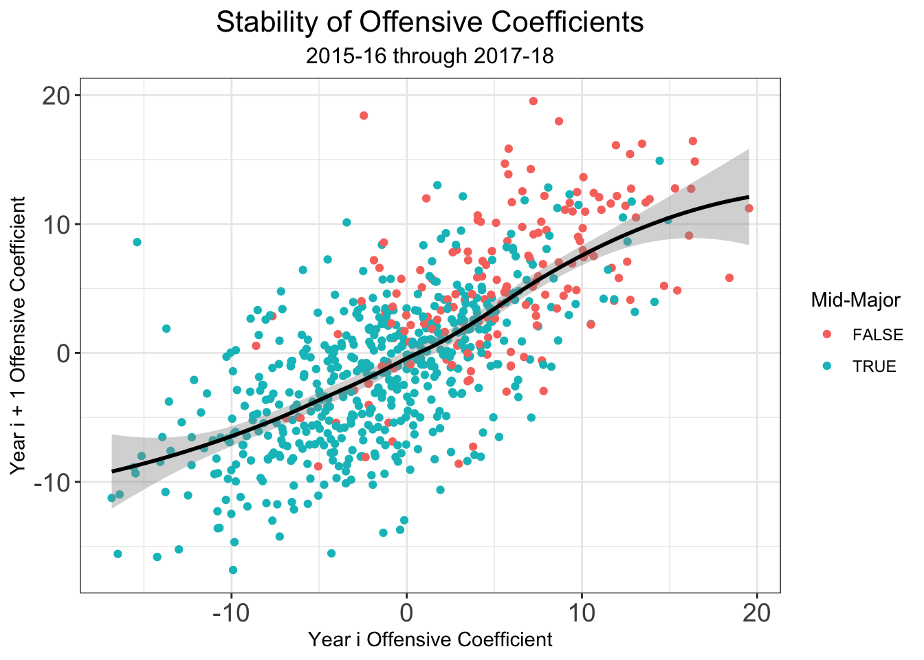
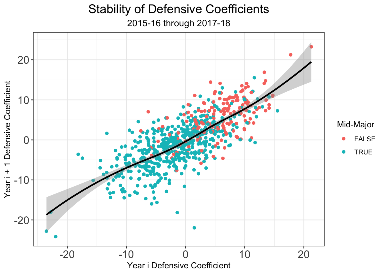
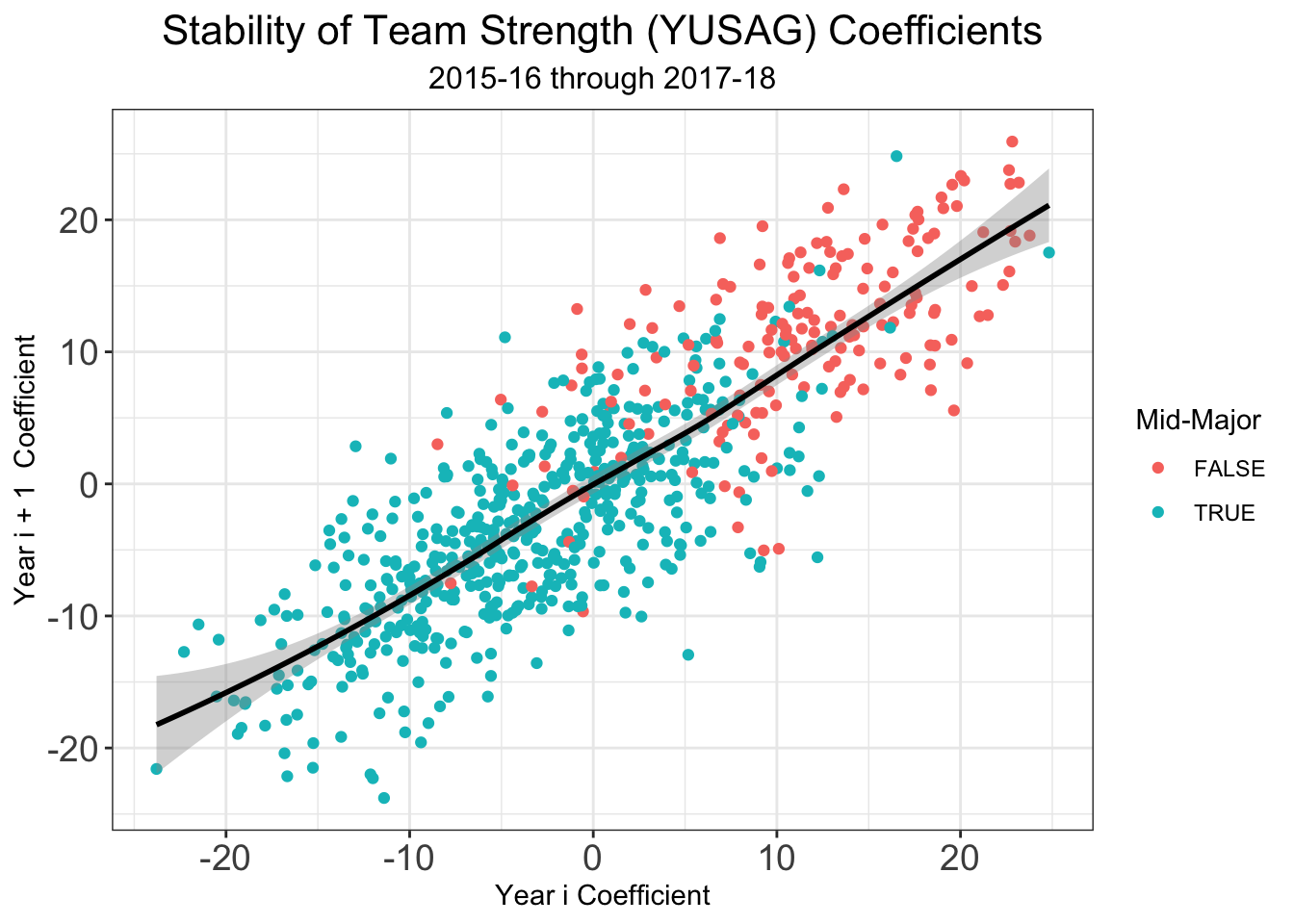
We see that there is higher year to year variability in the offensive coefficients than in the defensive coefficients. So if we can account for some of the year to year variation due to some of the factors surrounding why a team’s roster from year to year, this can help us set good preseason ratings. While my system doesn’t make use of individual player data in-season, I think that it allows us to extract the most information out of how teams change from year to year. All of the the individual level data was graciously given to me by Bart Torvik, who honestly has one of the coolest sites on the internet if you’re a college hoops fan. Bart keeps track of a player value metric called, “Points Over Replacement Player Per Adjusted Game At That Usage”, or more simply PPG! . Examining returning players who played at least 40% of possible minutes for their teams, I computed team level returing PPG!, departing PPG!, and incoming transfer PPG! . Additionly, Bart provided me with team level percetange of returning minutes. Combining that with my own recruiting data pulled from 247Sports.com, I used the several variables to predict offensive and defensive coefficients from the the previous years statistics. Regressions were fit on data 2015-16 \(\rightarrow\) 2016-17 and 2016-17 \(\rightarrow\) 2017-18 using 10-fold cross validiation. The following variables comprised the models.
\(\alpha_{team}^{\text{year =} i+1}\)
- \(\alpha_{team}^{\text{year =} i}\)
- 247Sports Composite Recruiting Score (for Incoming Recruiting Class)
- Returning PPG!
- Departing PPG!
- Indicator for having at least 1 5-Star Recruit
- Indicator for having at least 3 5-Star Recuits
- Indicator for having at least 3 3-Star, 4-Star or 5-Star Recuits
Model \(R^2 = 0.59\)
\(\delta_{team}^{\text{year =} i+1}\)
- \(\delta_{team}^{\text{year =} i}\)
- 247Sports Composite Recruiting Score (for Incoming Recruiting Class)
- Returning PPG!
- Departing PPG!
- Indicator for having at least 3 5-Star Recuits
Model \(R^2 = 0.59\)
From this, not only get a much improved preseason estimate of a team’s true strength (\(\hat \gamma_{team} = \hat \alpha_{team} + \hat \delta_{team}\)), but we can also get a prior distribution on the these coefficients as well, utilizing the variance of \(\hat \gamma_{team}\). Perhaps not suprisingly, the uncertainty in these distributions is greater for teams with more high level recruits and fewer returning players. Compare the following preseason priors for some of the more interesting teams this year.
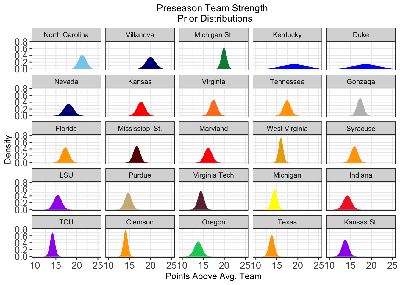
Let’s take a look at the top-25 teams heading into the 2018-19 season.
##               team yusag_coeff
## 1   North Carolina    21.29206
## 2        Villanova    20.00146
## 3     Michigan St.    19.94314
## 4         Kentucky    19.14156
## 5             Duke    18.63643
## 6           Nevada    18.04865
## 7           Kansas    17.74140
## 8         Virginia    17.46613
## 9        Tennessee    17.42049
## 10         Gonzaga    17.28193
## 11         Florida    17.25448
## 12 Mississippi St.    16.70156
## 13        Maryland    16.18948
## 14   West Virginia    15.95730
## 15        Syracuse    15.93676
## 16             LSU    15.42715
## 17          Purdue    14.68644
## 18   Virginia Tech    14.44185
## 19        Michigan    14.42888
## 20         Indiana    14.25695
## 21             TCU    14.19995
## 22         Clemson    14.05680
## 23          Oregon    13.80570
## 24           Texas    13.77246
## 25      Kansas St.    13.74995
Lastly, I should make comment on how rankings were detemined for the two new teams to Division 1 this season, Cal-Baptist and North Alabama. Given that much of these preseason rankings depends on end of season rankings from last year, setting prior rankings for Cal-Bapist and North Alabama required imputing missing values. I looked at the correlation betwen my preseason offensive and defensive coefficients with T-Rank adjusted offensive and defensive efficiencies. Perhaps I’m beating a dead horese here is reminding the reader that my own coefficients are not measures of efficiency, and one might wonder then why I’d use adjusted efficieny margins to impute preseason rankings for these schools. Overall, even though my coefficients and Bart’s rankings have different interpretations, there is a high correlation, and as such, this gives me a quick and dirty way to impute the preseason ranking for 2 of the 353 D1 teams. Using this imputation yields the following results
##   rank               team off_coeff def_coeff yusag_coeff
## 1  338         North Ala. -8.554625 -3.560665   -12.11529
## 2  346 California Baptist -8.554573 -5.105342   -13.65992
In-Season Updating
Let \(\alpha_{prior}, \delta_{prior}\) and \(\gamma_{prior}\) denote a team’s prior season coefficients. We’ll also obtain coeffient estimates from the current season’s games that have already been played, using least squares regression model explained above. I’ll note that in fitting this in-season model, I actually use weights to add a little bit of recency bias. That is, games that have been played are weighted more heavily. Suppose Team A and Team B played a game. It was the \(i^{th}\) game of the season for Team A and and the \(j^{th}\) game of the season for Team B. Furthermore, suppose that Team A has played \(n_a\) games to date and Team B has played \(n_b\) games to date. We define the relative recency of a game, \(r\) as follows.
\[
r = \frac{1}{2}\biggl(\frac{i}{n_a} + \frac{j}{n_b}\biggr)
\]
Finally, the games weight in the model is given by
\[
w = \frac{1}{1 + 0.5^{5r}e^{-r}}
\]
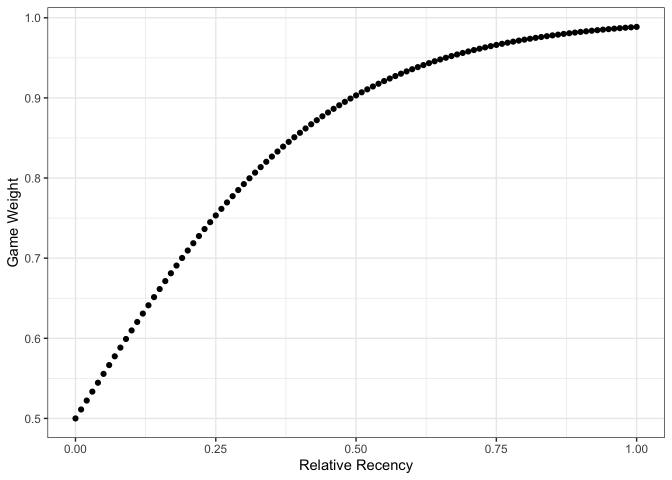
This bias really only downweights early season games when the majority of the season has already been played.
Ok so now that we have coefficient estimates for each team prior to the season and estimates from the current season’s worth of data what do we do? Part of the reason the preseason ratings of interesting is that estimates of team coefficients are extremely noisy early in the season. To get around this, we can take a weighted average of a team’s in-season coefficients and preseason coefficients. Suppose a team has \(n\) games on it’s schedule, and it’s most recent game played was the \(k^{th}\) game on the schedule. Then we have \[ w = \min\biggl(\frac{2k}{n}, 1\biggr) \] \[ \gamma_{team} = w\gamma_{in\_season} + (1-w)\gamma_{pre\_season} \]
Note that we do the same as above for \(\alpha_{team}\) and \(\delta_{team}\). Preseason weights fall out completely once a team completes \(\frac{1}{2}\) of it’s schedule, as the halfway point is roughly the point in the season by which coefficient estimates begin to stablilize. One might wonder why not take a full Bayesian approach to get posterior distributions for model coefficients. I’m hesitant to take a full Bayesian approach is that the I’m fairly confident my uncertainty estimates are underestimates, meaning these preseason priors would be too informative. I think that after spending this season evaluating the current framework, I’d feel more comfortable setting weaker priors around similarly obtained point estimates to establish a Bayesian framwork. That’s definitely the direction this project is headed but I have to make sure I wouldn’t be setting terrible priors before making such a switch.
For full 1-353 rankings, click here. Code for this model will be updating shortly here
Acknowledgements
I can’t finish this post without thanking Bart Torvik one final time. Bart provided me with a lot of his proprietary data over the summer and answered many many questions I had in setting priors. Be sure to check out his site if you haven’t yet!