Introduction
This summer brings the competition of the UEFA Euro Cup and COPA America, the European and South American (+ select North American) continental soccer championship. Outside of the World Cup, these are the two pinnacles of international soccer. As I have done for previous soccer tournaments, I’ve decided to model and simulate each of these major tournaments. Results of 10,000 simulations of each tournament are below. For the curious reader, I’ve specified some model details and linked to code repositories at the end of this article.
I’ll try to update these predictions throughout the tournament but I’m most likely to be discussing them on Twitter so check there to follow along.
Euro 2024
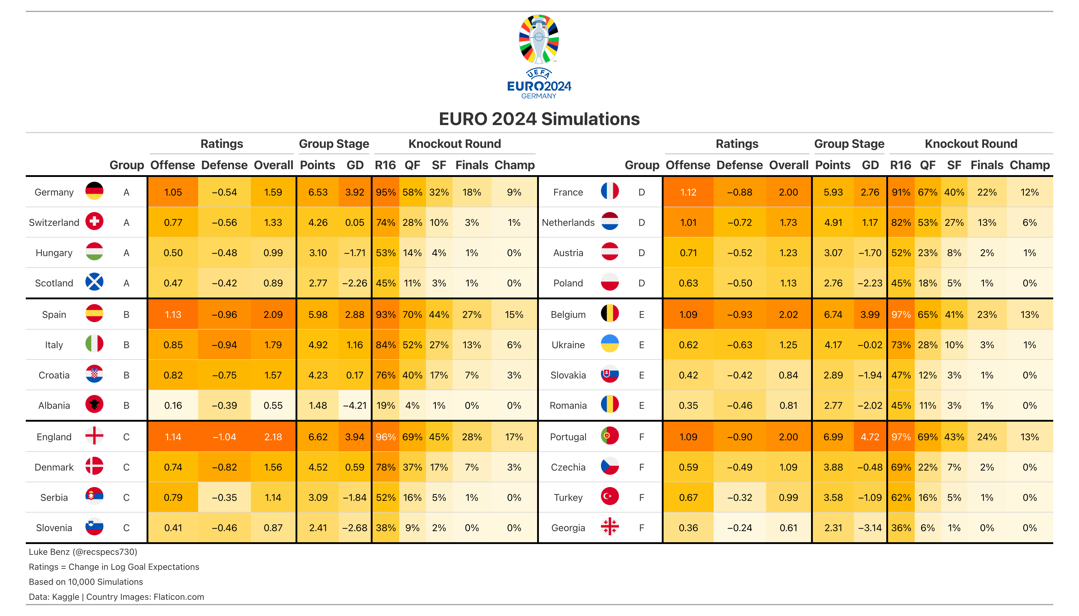
- England is the favorite at 17%, followed by Spain at 15%
- Portugal is 3nd favorite at 13%, benefiting from a very easy group on paper
- My model is a bit lower on France than betting markets, as I have them at just 12% to win. I think it’s partially a function of a very challenging group draw.
Copa America 2024
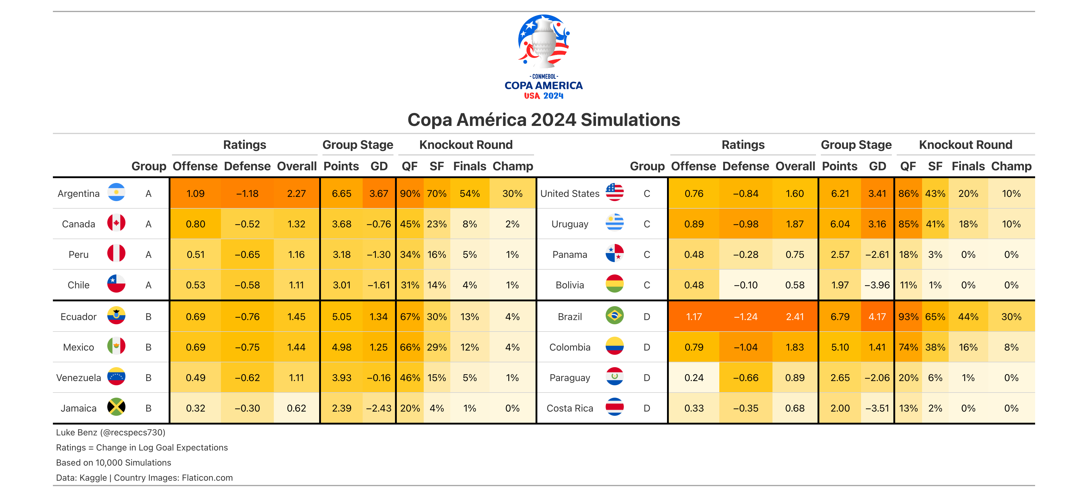
- No surprises here, Brazil (30%) and Argentina (30%) are co-favorites and likely to meet in the finals.
- United States has a 10% chance to win, which I guess is pretty good given when US Soccer has been lately. They benefit from hosting the tournament as well as the fact that it’s a small tournament.
- For some reason Groups A/B can’t play Groups C/D until the finals which means we’re likely to have some rematches in the semi-finals.
The Model
The model used in these simulations is slight variation of the Bayesian bivariate Poisson model (BVP) outlined in Equation (2) of (Benz and Lopez, 2021). The BVP modeling framework is as follows. Let \((Y_{ij}, Y_{ik}) \sim BVP(\lambda_{1i}, \lambda_2, \lambda_3)\) denote the goals for two teams \(j\) vs. \(k\) in match \(i\). Under this framework, \(Y_{ij} \sim \text{Pois}(\lambda_{1i} + \lambda_{3i})\) and \(Y_{ik} \sim \text{Pois}(\lambda_{2i} + \lambda_{3i})\), where \(\lambda_{3i}\) can be viewed as a correlation term between the expected goals for the two teams in game \(i\). In our previous work, we found that goals are better modeled w/ \(\lambda_3 = 0\), a finding similar to that of (Groll et al. 2018). Adopting this choice for this work, this reduces to a product of two independent Poisson random variables, which I model as follows:
\[ \begin{aligned} \log(\lambda_1) &= \mu + \alpha_{t[j]} + \delta_{t[k]} + \biggr(\tau_{h}\mathbb{I}(j = \text{home})~+~\tau_n\mathbb{I}(j = \text{neutral})\biggr) \\ \log(\lambda_2) &= \mu + \alpha_{t[k]} + \delta_{t[j]} + \biggr(\tau_{h}\mathbb{I}(k = \text{home})~+~\tau_n\mathbb{I}(k = \text{neutral})\biggr) \\ \end{aligned} \] In the above,
- \(\mu\) represents the log goal expectation of an average international team playing away from home
- \(\alpha\) represents attacking team strengths
- \(\delta\) represents defensive team strengths
- \(\tau\) represents location parameters. In the majority of games in these tournaments, the games will be neutral site. For the respective hosts however, home teams get a slight boost.
It would be nice to estimate country or tournament specific home advantage parameters but there aren’t really enough historical data points to do this.
One of the challenges of modeling these types of tournaments is that international don’t play very many games per year, and when they do play, many of the games are international friendlies not part of any competition, so it’s hard to gauge how seriously to take those results. Thus, I’ve added some additional observation weights to the log-likelihood when fitting this model in STAN. Specifically, each game is weighted as follows
\[ w_i = b_i\exp\biggr(-\frac{T_\max - T_i}{T_\max-T_\min}\biggr) \]
- \(b_i\) is the base weight for game \(i\) which is 1 for friendlies, 1.25 for Nations League Games, and 2 for continental championships/World Cups.
- \(T_i\) is the date of game \(i\)
- \(T_\min\) and \(T_\max\) are the earliest/latest games in the same I am using
The \(\exp(\cdot)\) term decays weights such that more recent games count more than older games. I restricted analysis to games from the start of 2018 onwards. \(T_\min\) and weights \(b_i\) are in theory tunable parameters that I chose somewhat arbitrarily. With more time, I’d do cross validation for these parameters but I have just chosen these for now and they seem reasonable.
I fit the model in Stan, and you can see more about prior choices or other model fitting choices in the code linked below.