As part of my thesis this past spring, I improved on the win probability built into my ncaahoopR package. The new win probability model has now been integrated into the package for the upcoming 2019-20 college basketball season. In this post, I provide some background on the statistical details of the model.
Win Probability Model Framework
Let \(p_{ikt}\) denote the probability that team \(i\) wins game \(k\) with time \(t\) remaining in the game. Let \(Y_{ik}\) be an indicator whether team \(i\) won the game \(k\). The following model is assumed: \[ \begin{aligned} Y_{ik} | p_{ikt} &\sim \text{Bernoulli}(p_{ikt}) \\ \text{logit}(p_{ikt}) &= X_{ikt}^{\scriptstyle T}\beta_t + \epsilon_{ikt} \\ \epsilon_{ikt} &\sim N(0, \sigma^2) \end{aligned} \] In the above model, observations are of the form $ X_{ikt}, Y_{ik})$, where $ X_{ikt}$ denotes a vector of covariates of interest with time \(t\) remaining in game \(k\) and, \(Y_{ik}\) is an indicator whether team \(i\) won \((Y_{ik} = 1)\) or lost \((Y_{ik} = 0)\) the game in question. \(X_{ikt}\) occur at discrete, non-regular time points \(t\), as observations are only available after the occurrence of certain game events (such as a made basket, foul, turnover, or timeout) which don’t adhere to a regular time schedule.
\(\beta_t\) represents the vector of coefficients for the covariates of interest with time \(t\) remaining. One challenge in fitting the above model is that the covariates of interest, such as score differential and pre-game point spread, have non-linear dependencies on the amount of time remaining in the game. While time remaining is not explicitly a covariate in any version of this model, coefficient estimates for covariates of interest are obtained at various values of time remaining \(t\). To combat covariates’ non-linear dependence on time, various versions of this type of college basketball win probability model, including work by Brian Burke and Bart Torvik have broken the game into discrete time chunks, over which the coefficients are assumed to be constant.
However, numerous problems can arise when one categorizes or makes discrete a continuous variable. To get around this problem, I fit several versions of this model were over discrete time intervals which overlapped by 90%. LOESS smoothing was then applied to the resulting coefficient estimates to obtain smooth coefficient functions over time. Coefficient estimates represent the increase in the log odds of winning a game while holding all of the other covariates in the model constant.
I trained and tested several variations of this kind of model, which you can read about here. The model ultimately settled on is as follows:
For each interval of the form \((t - \Delta, t]\), a logistic regression fit with covariates Pre Game Point Spread (favored_by) and Score Differential (score_diff) such that \(t - \Delta \leq\) time_remaining \(\leq t\). Consecutive intervals overlap one another by 90%. As the time remaining, \(t\) approaches \(0\), the rate at which model coefficients change with time increases. As such, \(\Delta\) is decreased in order to properly capture the manner in which these coefficients vary as a function of time.
| Variables Included | Time Interval Structure \((t - \Delta, t]\) |
|---|---|
|
|
Essentially, this method is related to a Generalized Additive Model (GAM). In simple terms a GAM is a linear combination of some unknown smoothed functions over the covariates. What I have done is essentially reverse the steps–I fit linear combinations of predictors (with logit link function) and then smooth over the time dependent results. This was done to gain a little bit more interpretability of the coefficient values, although I think a GAM could be fit and obtain vary similar results.
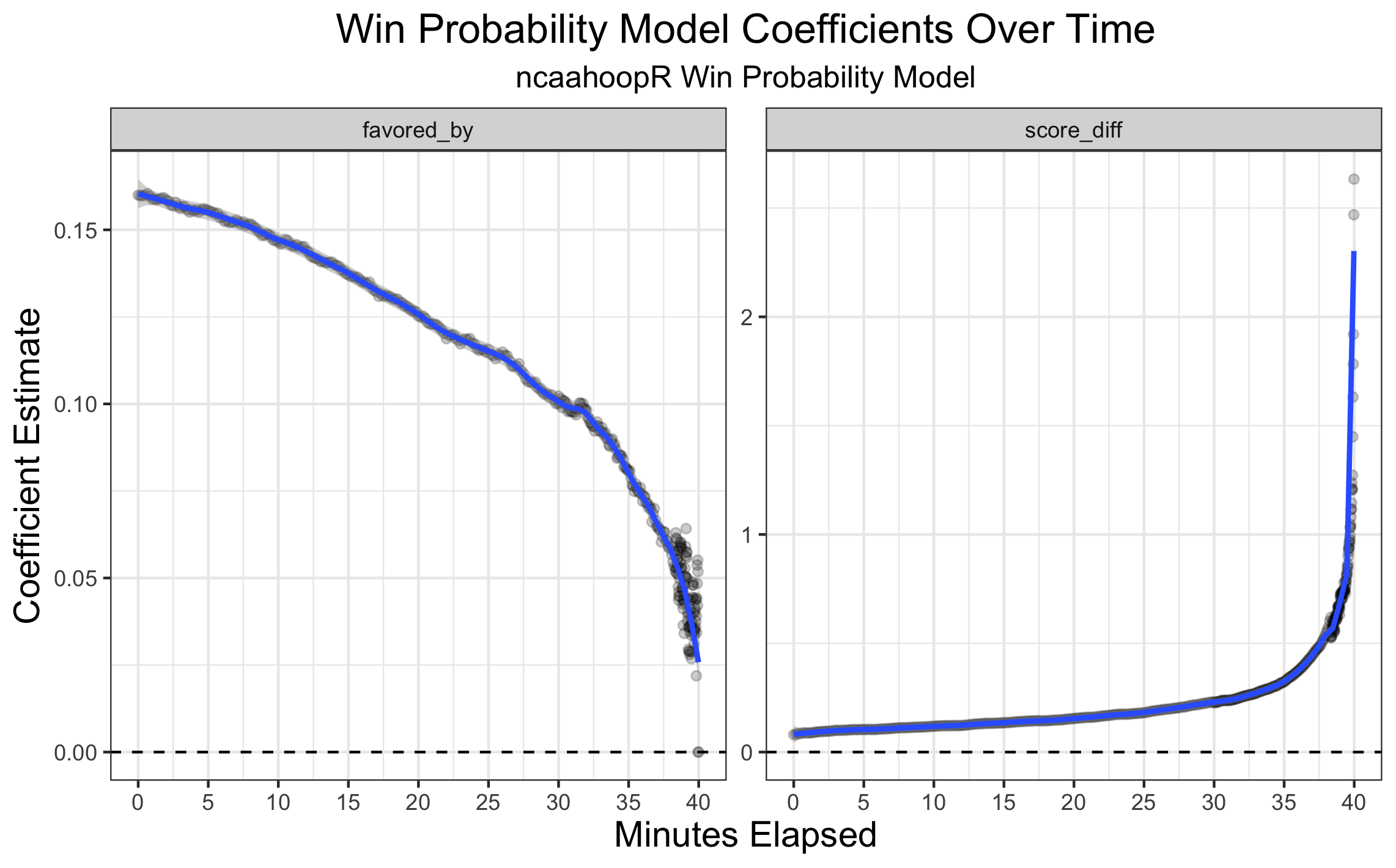
We see in the coefficient trace plot below the obvious result that as the game progresses, the pregame line becomes less important in predicting win probability and the current score differential becomes increasingly more important
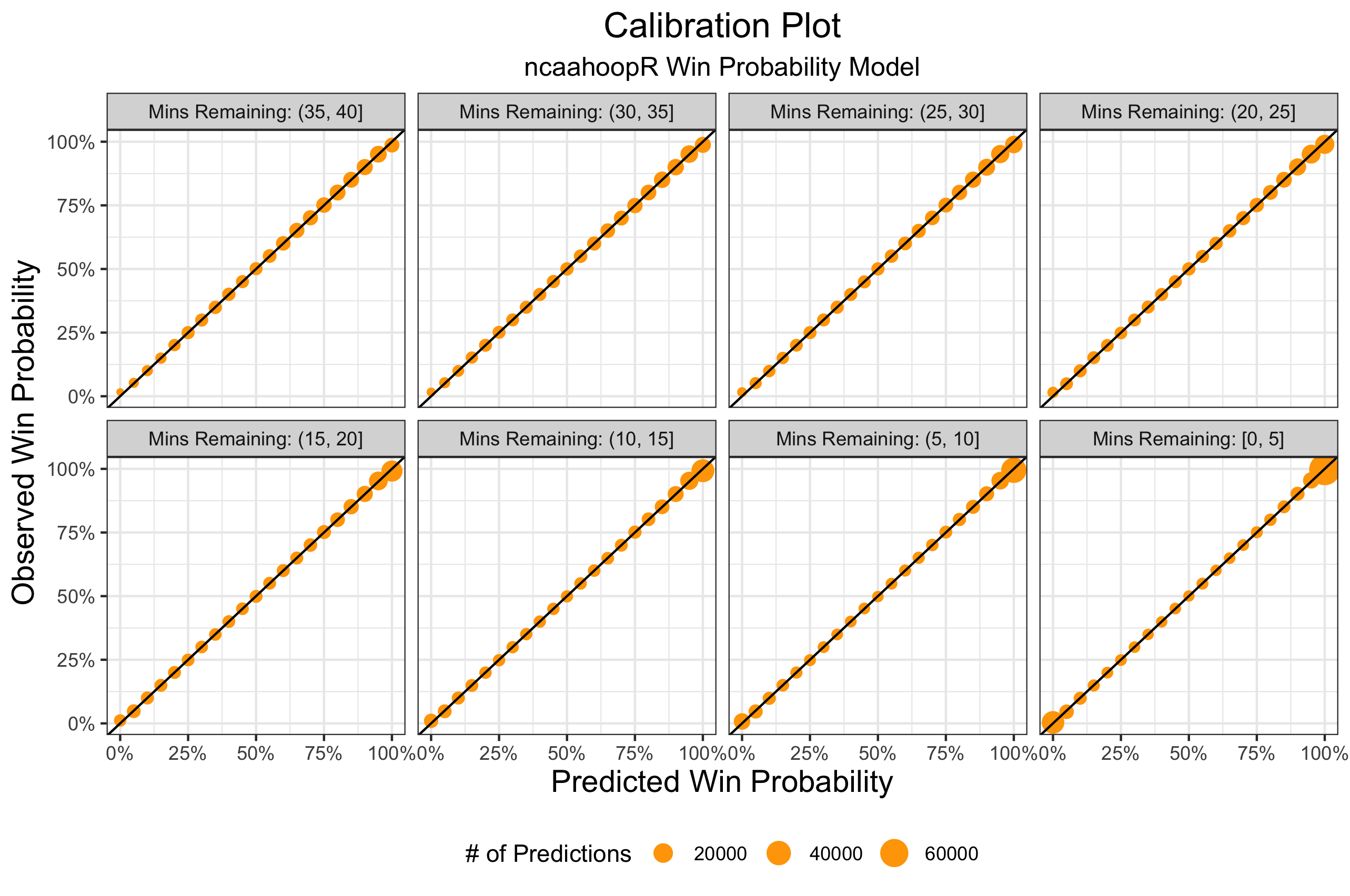
Model Calibration
The model above was trained on 10,949 games from the 2016-17 and 2017-18 seasons and tested on 3,625 games from the first part of the 2018-19 season. Using the idea of calibration plots from Michael Lopez’s win probability post after the 2017 Super Bowl, I compare bins of predicted and observed probability over the course of the game. We see that the model is well calibrated for all situations.
Summary
Compared to the older win probability model, the new win probability model is smoother and a little bit more interpretable. It is trained on a larger sample of data and is better calibrated, especially in late game situations. I still think there are some improvements that can be made in the future, especially accounting for possession in the final few minutes of the game. Nevertheless, it’s nice to see something fairly simple performing so well, and to integrate something I worked on for my thesis into the package. Be on the lookout for new win probability charts dropping at the beginning of this season!