Introduction
With the 2018 FIFA World Cup nearly upon us, we set out to build a model to predict game outcomes and estimate coutries chances of reaching various rounds of the tournament. Ranking systems for various sports, including NCAA Men’s Basketball, NCAA Football, and NBA, have been the basis of several of our projects in the past. With the exception of rankings using ELO, all of our past ranking systems have made use of linear regression in one form or another. Simply, those models took on something similar to the following form
\[
Y = \beta_0 + \beta_{team} X_{team} + \beta_{opp} X_{opp} + \beta_{loc} X_{loc} + \epsilon
\]
where \(X_{team, i}, X_{opp, i}\), and \(X_{loc, i}\) are indicator vectors for the \(i^{th}\) game’s team, opponent, and location (Home, Away, Neutral) from the perspective of team, and \(Y_i\) is game’s the score-differential. The key assumptions for this model are that game outcomes are independent of one another, and that our error \(\epsilon \sim N(0, \sigma^2)\).
First Attempt
Before going into detail on the model we ultimated settled on, let’s first examine what didn’t work–and more importantly why. Given our prior experience using linear regression to predict score differential in several different sporting events, it seemed natural to extend the notion to international soccer. In fact, our initial attempt seemed quite reasonable. The basic idea was as follows:
- Use linear regression with covariates
team,opponent, andlocationto predictgoal_diff(a game’s goal differential). - Use a multinomial logistic regression model with input
pred_goal_diffto estimate probabilities ofwin,loss, andtie. Our rankings indicated that Germany, Brazil, and Spain were the top 3 teams, entirely plausible our eyes (as casual soccer fans).
In writing Monte Carlo simulations to estimate round-by-round probabilities of advacing, we began to notice a potential fault in our model. While it was easy enough to simulate game outcomes and award points (3 for win, 1 for tie, 0 for loss) given our estimated win, loss, and tie probabilites for each of the group stage games, breaking ties in the group standings to determine which two teams would advance to the knockout round presented more of a challenge. If two or more teams are tied on points after a round robin within the group, the first tie-breaker is net goal differtial, a country’s goals scored - goals allowed in the 3 group stage games. Our initial thought was to simply flip a coin to break ties, but this underestimates the probabiity that better teams advance past the group stage. Consider the following hypothethical scenario in group B:
| Spain | 9 | |
| 2 | Portugal | 4 |
| 3 | Morocco | 4 |
| 4 | Iran | 0 |
Simply flipping a coin to determine whether Portugal or Morocco would advance in the above case almost certianly underestimates the chances that Portugal, the superior of the two, would have a larger goal differential than Morocco. So, was there a better way to account for goal differntial? Recall, goal_diff was the response variable of our linear regression. A nice result of simple linear regression is that for game \(i\), we have \(\widehat Y_i\) normally distributed. Since \(\widehat Y_i = \widehat \beta_0 + \widehat\beta X_i\) and each \(\widehat \beta_i \sim N(\beta_i, \sigma_i^2)\), \[\widehat Y_j \sim N(\beta_0 + \beta X_j, \sum_i \sigma_i^2)\]
Approximating such a distribution using prediction intervals for goal_diff, perhaps we could form net goal differential distributions for each team in group play and randomly draw from those distrubutions in the case of a tie in the group standings. Things quickly became not well-defined when trying to draw from \(Y \sim N(\mu, \sigma^2) | Y \geq 1\) (in case of loss, \(Y \leq -1\)). Moreover, in the case of a tie, we’d be setting \(Y = 0\) in our simulation, yet under the normal distribution, \(P(Y = 0) = 0\) (in fact the probability \(Y = c\) exactly is 0 any fixed constant \(c\)). By this point, we’d realized we were in trouble, as drawing from this continuous distribution for a discrete random variable didn’t make a lot of sense. Back to the drawing board.
Taking a Step Back
At this stage, there are two questions to consider. The first, is why didn’t a linear model, which had worked well for us in the case of basketball and football, work well in the case of soccer? Furthermore, we wondered, if not a linear model, what type of model would work best? The answer to both of these questions is best seen by looking at histograms of points/goals scored in soccer games vs. basketball games.
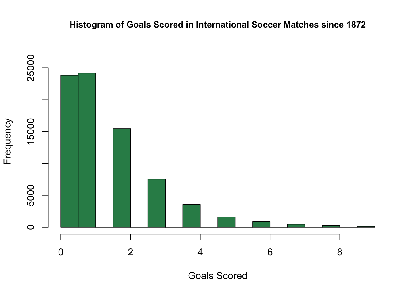
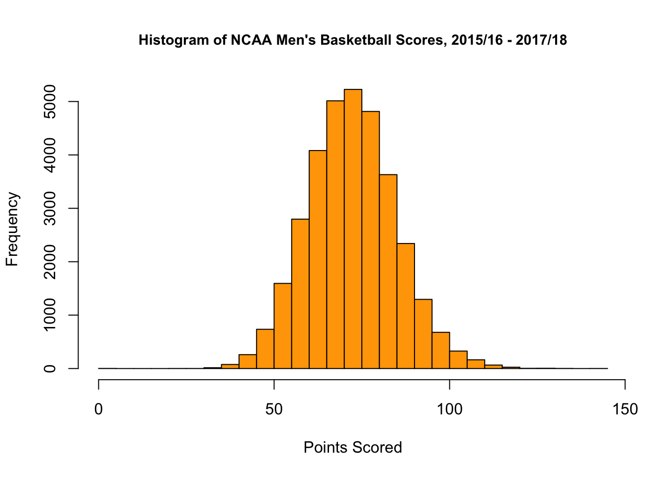
Based on the plots above, we see that the distribution of basketball scores looks like a bell curve, while the distribution of soccer scores does not. Rather, the distribution of soccer scores looks to be more like a Poisson distribution. Recall that the probability mass function (PMF) of the possion distribution with parameter \(\lambda\) is by \[ P(X = k) = \frac{e^{-\lambda}\lambda^k}{x!} \textrm{ for } x = 0, 1, 2, ... \]
Additionally, if \(X \sim Pois(\lambda)\), \(\mathbb{E}(X) = \lambda\). As \(\lambda\) gets large, Poisson distributions become more and more like Guassians, hence the ability for sports with larger average scores (i.e. basketball) to be better modeled with a Normal Model than sports with lower scores (i.e. soccer, hockey). Since the difference of i.i.d. normal random variables is also normal, linear regression is perfectly fine for modeling score_diff is basketball. However, the difference of two i.i.d. poisson random variables is not normal nor poisson. Rather, the difference of two poisson random variables follows the skellam distribution. Thus, it seems like our best bet here is to use poisson regression for our model. In fact, several studies have shown that poisson regression is good for modeling soccer 1 2 3 4.
Building the Model
The data, available on Kaggle, covers over 39,000 international soccer matches dating back to 1872. For the purpose of this model, we have chosen to use data for games played after January 1, 2014. Many major tournaments in soccer, the World Cup included, occur on a four year cycle, so using the last 4 years worth of data seemed natural.
Daniel Sheehan has written a fantastic blog post on using poisson regression to predict the outcomes of soccer games, and our model is based off of his work (he provides lots of examples in both R and Python, and we’d highly recommend reading it!).
We began by duplicating the data set and transforming one copy to be from the perspective of the opponent. For example, if we had the vector in the < team = "Germany", opponent = "Brazil", location = "N", team_score = 7, opp_score = 1 >, we’d also add to our data set the vector <team = "Brazil", opponent = "Germany", location = "N", team_score = 1, opp_score = 7 >. What we eventually end up predicting is team_score as a function of team, opponent, and location.
Before actually building the model, there were one more things that we considered, namely match_weight, how much weight we should give a particular game. There were two factors on which the model weights were set: time since the was played, and the type of match being played. We broke matches in our data set into four types (derived from the official FIFA rankings formula):
- Friendlies and other matches (Base Weight \(\alpha_i = 1\))
- Qualification matches for World Cup and continental championships (Base Weight = \(\alpha_i = 3\))
- Confederations Cup and continental championships (Base Weight = \(\alpha_i = 5\))
- World Cup Matches (Base Weight = \(\alpha_i= 8\))
Letting \(\delta_i\) represent the date on which game \(i\) was played and let \(\delta_t\) be today’s date (i.e. the date we choose to fit/re-fit the model). Finally, take \(\delta\star = \max_{i} (\delta_t - \delta_i)\). Then, the match_weight, \(w_i\) of match \(i\) is given by
\[
w_i = \alpha_i \times e^{- \frac{\delta_t - \delta_i}{\delta\star}}
\]
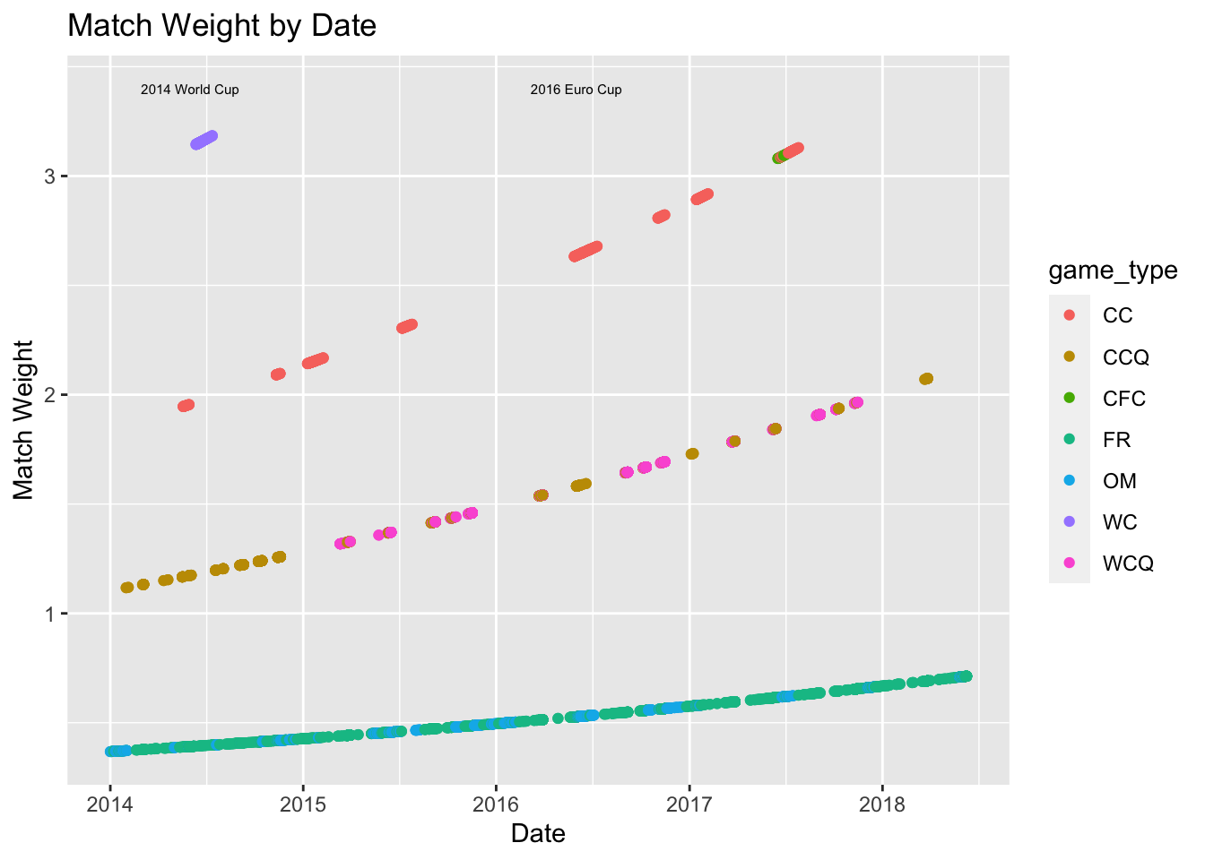
We see above that the 2014 World Cup and the 2016 Euro Cup are among the most heavily weighted games, as we would hope. Now the call to the model is as follows:
glm.futbol <- glm(goals ~ team + opponent + location,
                  family = "poisson",
                  data = y,
                  weights = match_weight)
The model gives coefficients for each country both as levels of the team and opponent factors. Since the model output predictions can be taken as the average team_score for a given team against a given opponent at a given location, we can view the country specific coefficients as offense and defensive components of a power rating. The interpretation of such coefficients is less intutive than in the case of linear regression, in which coefficients signfy points better than an average team, but you can think of them as more similar to logistic regression coefficients. Higher offensive coefficients indicate a team is likely to score more goals on average while low (more negative) defensive coefficients indicate a team is likely to conceed fewer goals on average.
##            team  offense   defense net_rating rank
## 77      Germany 1.707366 -1.373929   3.081295    1
## 72       France 1.581282 -1.307218   2.888500    2
## 29       Brazil 1.727649 -1.097520   2.825169    3
## 181       Spain 1.639751 -1.116924   2.756675    4
## 9     Argentina 1.318170 -1.438423   2.756593    5
## 45     Colombia 1.456873 -1.285449   2.742322    6
## 20      Belgium 1.565169 -1.140337   2.705506    7
## 140 Netherlands 1.597657 -1.065459   2.663115    8
## 158    Portugal 1.442856 -1.200933   2.643789    9
## 64      England 1.269063 -1.281223   2.550285   10
Offensively, the top teams by our model, are Brazil, Germany and Spain, while Argentina, Germany, and England posses the best defenses.
Sample Match Prediction
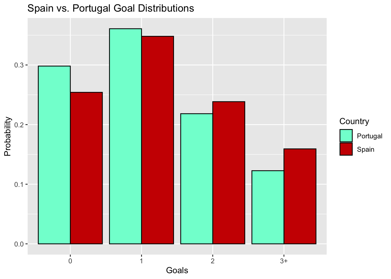
To see how this model works in more detail, let’s walk through how we predict the outcome of a single match. We’ll use the marquee Spain-Portugal fixture from Group B as our case study. The model output for the vector <team = "Spain", opponent = "Portugal", location = "N" > is 1.37, while the model output for the vector <team = "Portugal", opponent = "Spain", location = "N" > is 1.21 . This signifies that on average, we expect Spain to score 1.37 goals and expect Portugal to score 1.21 goals. There is much more information encoded in these two numbers however. Let \(X_s\) be the random variable denoting the number of goals Spain score and let \(X_p\) denote the number of goals that Portugal scores. Then, we have that \(X_s \sim Pois(\lambda_s = 1.37)\) and \(X_p \sim Pois(\lambda_p = 1.21)\), and from these distributions, we can get a lot of neat stuff. First, we can look at the joint distribution of goals scored. Rows indicate the number of goals Spain scores while columns correspond to the number of goals Portugal scores.
| 0 | 1 | 2 | 3 | |
|---|---|---|---|---|
| 0 | 0.0758 | 0.0917 | 0.0555 | 0.0224 |
| 1 | 0.1038 | 0.1256 | 0.0760 | 0.0307 |
| 2 | 0.0711 | 0.0860 | 0.0521 | 0.0210 |
| 3 | 0.0325 | 0.0393 | 0.0238 | 0.0096 |
Perhaps unsuprisingly, the most likely outcome is a 1-1 draw, but there is still about an 87% chance we see a different outcome. Summing the diagonal entries of this matrix (extended out beyond 3 goals–let’s assume it’s neither team will score more than 10 goals) gives the probability that that Iberian neighbors end in a stalemate, while summing the entries above the diagonal or below the diagonal yield Portugal or Spain’s chances of winning, respectively. Overall, we estimate that Spain has about a 41% chance to win, Portugal has about a 33% chance to win, and there is a 26% chance the two teams draw.
Simulating the World Cup
Now that we have the ability predict any game, we can run some Monte Carlo simulations to estimate the probability of each time winning the World Cup. We run 10,000 iterations of the following simulation steps:
- Simulate each group game by drawing the number of goals scored by each team from their respective poisson distributions.
- Advance the top 2 teams in each group by points, and in the case of ties, use goal differential, goals forced, and goals allowed (in that order) as tiebreakers.
- Simulate knockout round games as in step 1. If there is a tie, flip a coin to determine who wins the simulated penalty shooutout (assuming that teams convert penalties at similar rates, this is not a decent approximation 5).
- Repeat step 4 until there is a champion
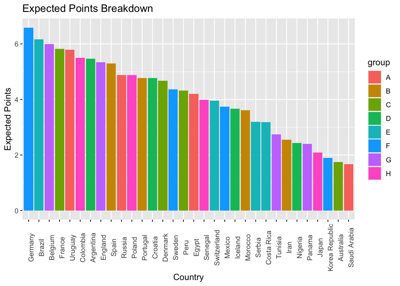
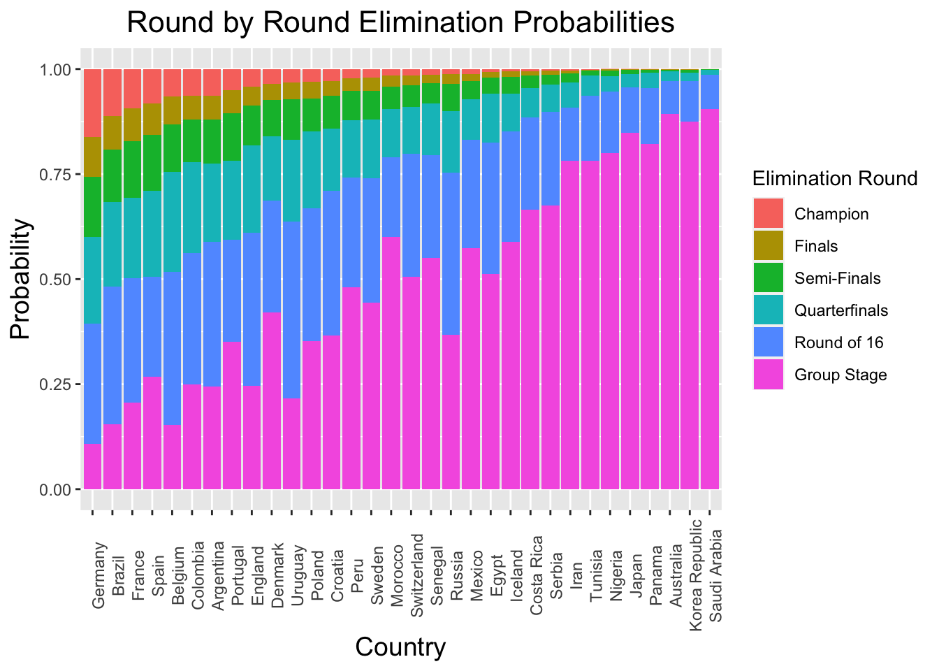
Our simulations indicate that despite being in the so called “group of death”, defending champion Germany is most likely to win the World Cup, with a roughly 16% chance to hoist the crown. Brazil (11%), Frace (9%), Spain (8%), and the trio of Argentina, Belgium and Columbia (6% each) follow closely behind. A full list of World Cup odds, as well as the code used in this project can be found on GitHub.
Limitations
A key assumption of the poisson distribution is that the rate parameter \(\lambda\) does not depend on time. That is, in using this model, we are assuming that the rate of goals is equal during each minute of the match. However, this is not true in practice, and several sources extend their framework to bivariate poisson regression 6 7 8 9. Other limitations include the relatively small number of important matches in international soccer. While we examine on a 4 year basis, there may only be 15-20 matches per team of the highest importance, making prediction dificult even with our best effort to correct for difference between matches on the basis of time and relative importance.
Acknowledgements
We’d like to thank Kostas Pelechrinis and Michael Lopez for offering suggestions regarding the switch from linear to poisson regression, as well as providing example papers modeling soccer outcomes using poisson regressions. Additionally, we’d like to thank Edward Egros, who mentioned the data set used in this project during his April visit to Yale University.
https://www.jstor.org/stable/4128211?seq=1#page_scan_tab_contents↩︎
http://www2.stat-athens.aueb.gr/~karlis/Bivariate%20Poisson%20Regression.pdf↩︎
https://fivethirtyeight.com/features/a-chart-for-predicting-penalty-shootout-odds-in-real-time/↩︎
https://www.jstor.org/stable/4128211?seq=1#page_scan_tab_contents↩︎
http://www2.stat-athens.aueb.gr/~karlis/Bivariate%20Poisson%20Regression.pdf↩︎